Use it in
Charts in Google Sheets.
=IMAGE() shows a chart inside a cell. Build the URL from your cells and the chart follows the numbers.
KPIsSheet 1
| A | B | C | |
|---|---|---|---|
| 2 | Jan | 1,180 | 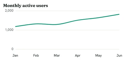 |
| 3 | Feb | 1,320 | |
| 4 | Mar | 1,290 | |
| 5 | Apr | 1,510 | |
| 6 | May | 1,640 | |
| 7 | Jun | 1,820 |
Set it up.

Size it for the cell
Use w=400&h=200, or the size of the merged cells you want it in.
Build the URL from cells
TEXTJOIN turns a column of numbers into the comma list the URL needs.
Wrap it in IMAGE
The cell shows the PNG. Change a number and the cell shows the new chart.
=IMAGE("https://c.renderchart.com/?key=KEY&type=line&w=400&h=200&smooth=1"
  & "&x=" & TEXTJOIN(",", TRUE, A2:A7)
& "&y=" & TEXTJOIN(",", TRUE, B2:B7)) =IMAGE("https://c.renderchart.com/?key=rc_pub_live_7Hq2mX9pLk4vN8sT1wEa&type=line &x=Jan,Feb,Mar,Apr,May,Jun &y=1180,1320,1290,1510,1640,1820 &title=Monthly%20active%20users &smooth=1 &w=400 &h=200 ") Worth knowing.
- Renders
- Each new set of numbers is one render. Opening the sheet again, or sharing it, comes from cache.
- Labels
- Keep labels short; 11px labels still read in a 400 x 200 cell.
- Key
- Anyone who can see the formula can see your public key. Use a short URL to hide it.